Blog Post 7

# Lasso Variable Selection
set.seed(902333)
ss <- DataframeName %>% select(SPREAD, SP500, GOLD, OIL, CHHUSD, JPYUSD, RGDP, UNRATE, IPI, 'Copper Price', 'Median Income', BCI, CCI, rec)
x <- model.matrix(ss$rec~., ss)
y <- ss$rec
cv_mod_ss <- cv.glmnet(x, y, alpha = 1)
plot(cv_mod_ss)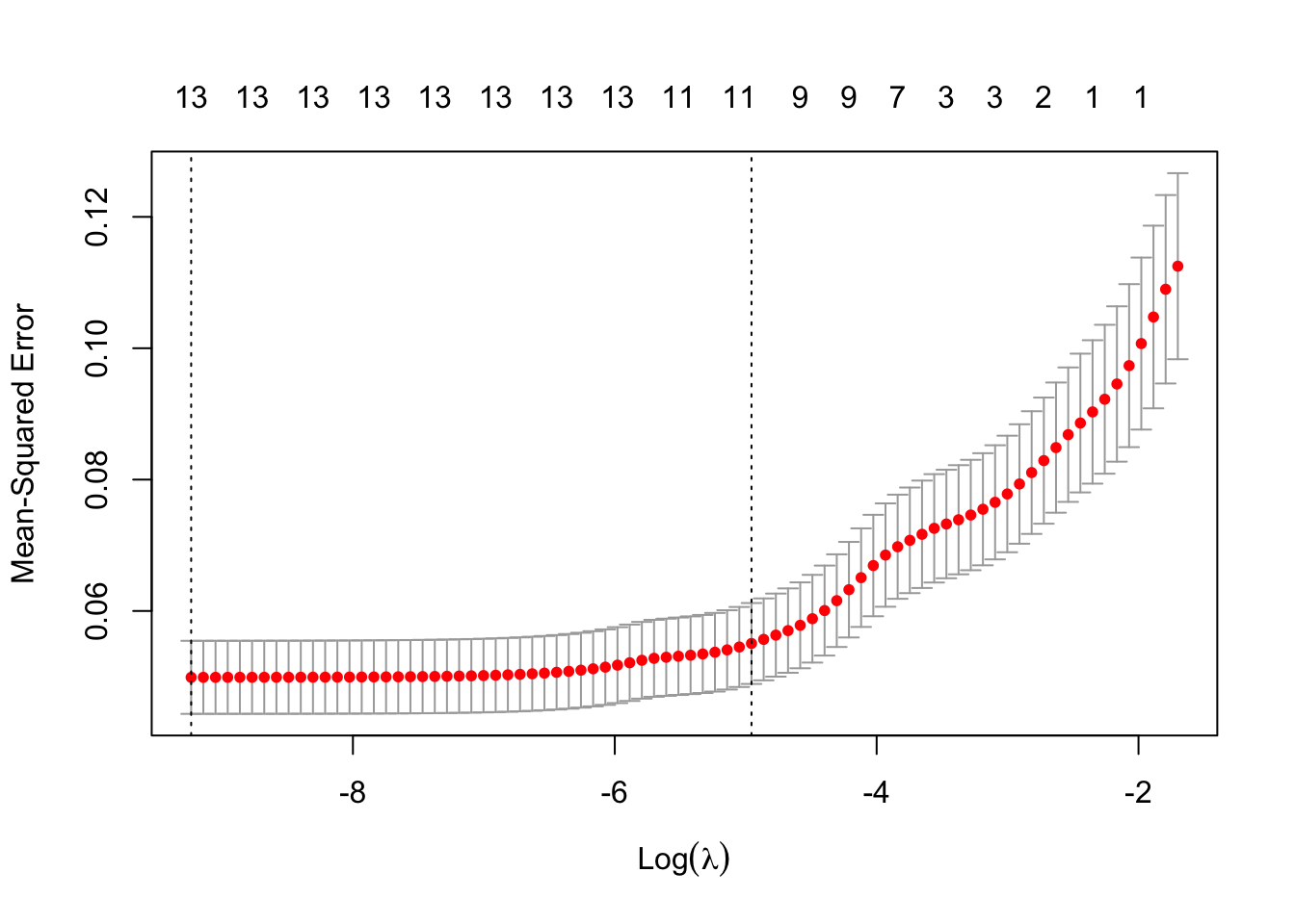

coef(cv_mod_ss)

## 15 x 1 sparse Matrix of class "dgCMatrix"
##                             1
## (Intercept)      2.057904e+00
## (Intercept)      .           
## SPREAD          -1.604249e-01
## SP500           -3.292787e-04
## GOLD             .           
## OIL              6.202401e-03
## CHHUSD           8.023310e-03
## JPYUSD           4.681710e-03
## RGDP            -6.660845e-02
## UNRATE          -6.025119e-02
## IPI             -2.088979e-03
## `Copper Price`   .           
## `Median Income`  3.160388e-05
## BCI             -3.574933e-02
## CCI              6.787614e-04

This week we finalized our variable selection process for our final model by using the Lasso method. We decided that the Lasso method was the best method for us, because we wanted to obtain a subset of predictors that minimizes prediction error for a quantitative response variable. From the figure, we see that 10 variables are significant and should be used in our final model. Besides this, we have also changed our front page picture and have started working on our interactive part of our project. Going into the final two weeks, we have a few things to do, but we are confident we can work together and produce a well rounded project.