Data Collection Procedure
The data we used for this project comes from various sources. Specifically, our data comes from a manicured Kaggle dataset, datasets from FRED, datasets from the Organization for Economic Co-operation and Development, and one dataset from a database server for Economic data called Macrotrends. We were able to find these datasets by searching for key indicators that affect recessions. For example, we would search for “Unemployment Rate”, and once the data was presented before us, we made sure the data contained “Unemployment Rates”, but also a time component. The time component in the datasets is crucial, because this is how we are able to combine our datasets and see the trends each variable has over time.
Main Datasets and Variables
This project consists of 14 variables. The three most relevant variables are our Recession Indicator, Real GDP, and Unemployment Rate. Additionally, for our project we only used CSV files, because we found CSV files to be the easiest type of file to work with and all of our datasets were in CSV data file type.
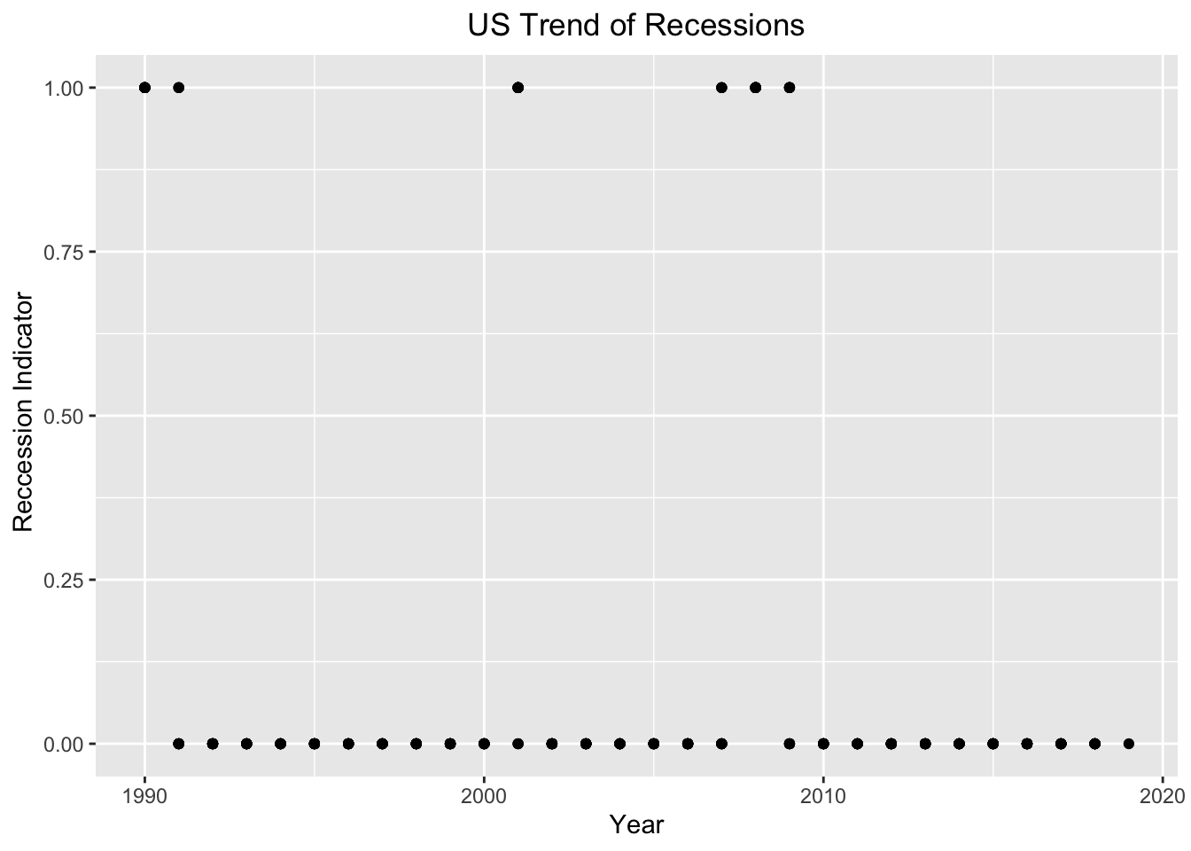
1. The dependent variable of our study is our Recession Indicator. The Recession Indicator is referred to as 1 during periods where a Recession was present in the US and 0 during periods where a Recession was not present in the US. The series assigns dates to US recessions based on a mathematical model of the way that recessions differ from expansions. The model indicates a recession whenever the GDP-based recession indicator index rises above 67%, the economy is determined to be in a recession. The date that the recession is determined to have begun is the first quarter prior to that date for which the inference from the mathematical model using all data available at that date would have been above 50%. The next time the GDP-based recession indicator index falls below 33%, the recession is determined to be over, and the last quarter of the recession is the first quarter for which the inference from the mathematical model using all available data at that date would have been below 50%. The Recession Indicator dataset was put together by James D. Hamilton, a Professor at the University of California San Diego, with ties to the National Bureau of Economic Research (NBER). The NBER are regarded as highly authoritative by academic researchers. The dataset was curated to follow and track the trends of Economics recessions.
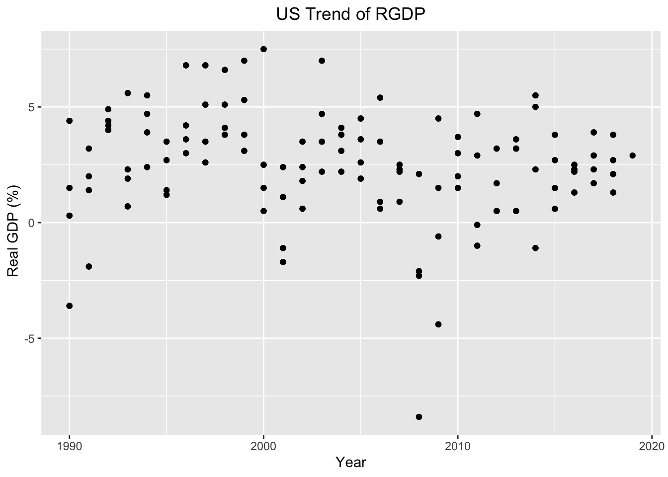
2. Real GDP is one of our important indicators, because Gross domestic product (GDP) is the value of the goods and services produced by the nation’s economy less the value of the goods and services used up in production. GDP is also equal to the sum of personal consumption expenditures, gross private domestic investment, net exports of goods and services, and government consumption expenditures and gross investment. Real values are inflation-adjusted estimates—that is, estimates that exclude the effects of price changes. The GDP dataset was put together by the US Bureau of Economic Analysis. The data was collected to track the trend of GDP in the US.
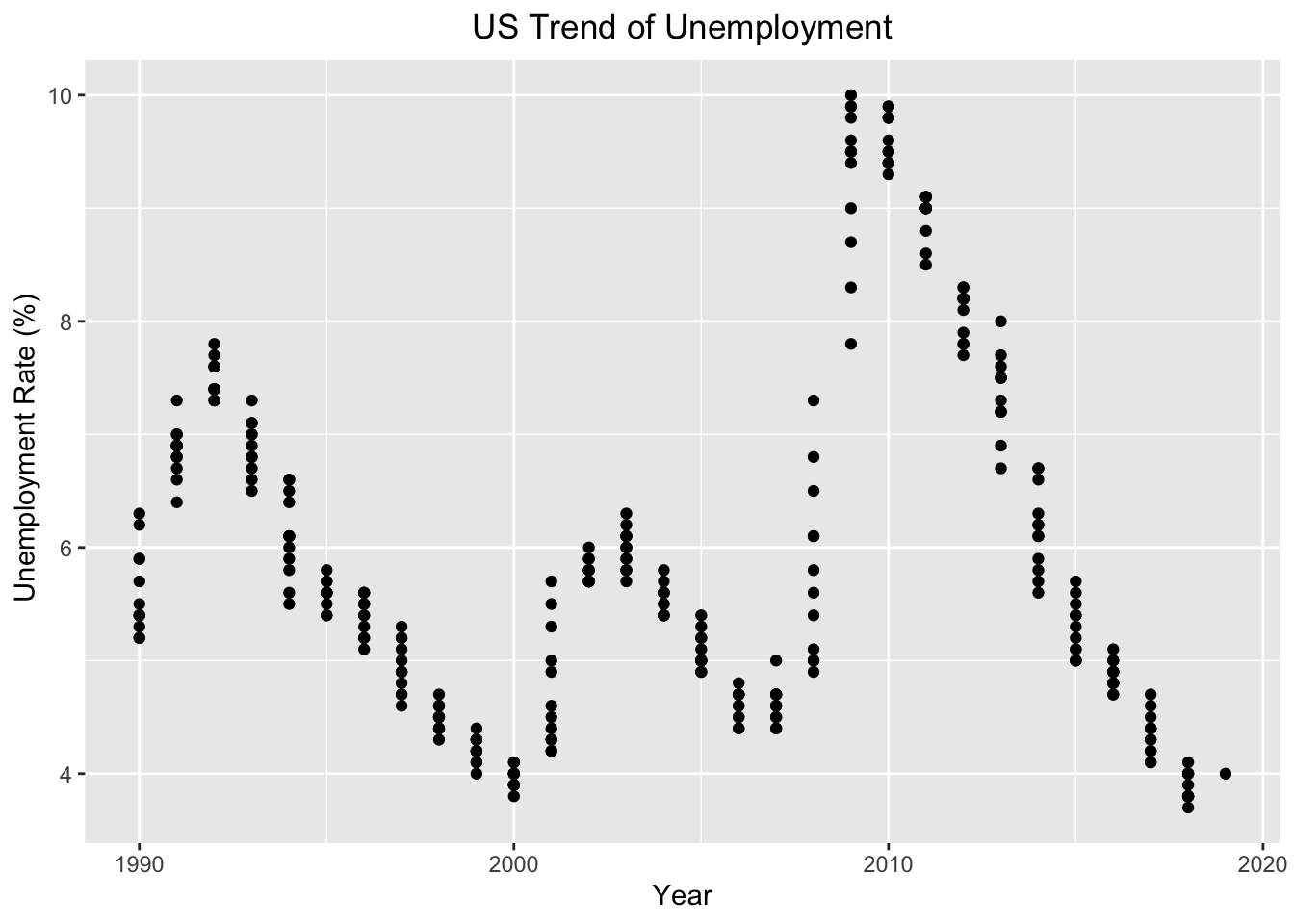
3. Unemployment Rate is another important indicator, because the unemployment rate represents the number of unemployed as a percentage of the labor force. Labor force data are restricted to people 16 years of age and older, who currently reside in 1 of the 50 states or the District of Columbia, who do not reside in institutions (e.g., penal and mental facilities, homes for the aged), and who are not on active duty in the Armed Forces. The Unemployment Rate dataset was put together by the US Bureau of Labor Statistics. The data was collected to track the trends of unemployment in the United States.
4. The remaining 11 variables includes median Income (Real median US household income), Business Confidence Index (Measure of Confidence within the industry sector), Consumer Confidence Index (Measure of confidence between consumers), Gold (price of gold), Oil (price of oil), Spread (the difference between the 30yr and 1yr maturities), SP500 (stock market index that tracks the stocks of 500 large-cap U.S. companies), CHFUSD (currency exchange rate for the U.S. dollar and swiss franc), JPYUSD (currency exchange rate for the U.S. dollar and Japanese yen), copper prices (price of copper), and Total Factor Productivity (measured as the ratio of aggregate output (e.g., GDP) to aggregate inputs). The majority of these variables comes from the Yield Curve Dataset. This dataset was put together by a journalist from Bloomberg, who was writing an article, “Is a recession coming? US Yield Curves can tell us”. However, we extracted this dataset from a Kaggle user named Andrada Olteanu, because the original datasource has a paywall. This dataset was collected, because Yield Curves are presumed to be good predictors of economic recessions. Another reason why this dataset was curated, was to assess how accurate Yield Curves can actually forecast recessions and when the next economic recession will take place.
Below are the links to these datasets.
Cleaning Data
To clean our data, we had to use two new libraries outside of what we learned. The two new libraries used to help us clean our data were zoo and anytime. The zoo library and anytime library both help us create and organize our time variable, so we could combine our datasets.
Here is a snapshot of our cleaning method.
# Mutating Date so we can join by date and look at date in various ways
yc <- yc %>%
  mutate(Date = ymd(Date)) %>%
  mutate_at(vars(Date), funs(year, month, day))

# Changing column names
colnames(rgdp)[colnames(rgdp) == "A191RL1Q225SBEA"] <- 'RGDP'

# Converting to correct datetime format
cci<-cci %>% mutate(Date = str_c(Date, "-01", sep= "",collapse =NULL)) %>% mutate(Date = anydate(Date))

# Making all datasets consistent to a monthly basis -> filling with dates and NA
rgdp <- rgdp %>% complete(Date = seq.Date(min(Date), max(Date), by="month"))

# Joining datasets
temp <- yc %>% inner_join(rgdp, by = "Date")
The above snapshot shows how we cleaned our data and combined our data. Every dataset had its own issues and required different techniques, so we could combined them. However, for almost all of the datasets we had to change the column names, so we could combined them. Additionally, some datasets required us to change their date format into our specific date format. Finally, we used an inner join to combine each dataset, so we could match the dates together and add the columns in the dataset we are joining by together.