
Our data analysis is motivated by looking at relationships between different economic indicators and whether or not a recession occurred. We are particularly interested in looking at inverted yield curves, unemployment rate, real GDP, and the S&P 500. Using logic and economic knowledge, we have ideas of how these indicators change in relation to a recession, for example we know real GDP drops when a recession happens. However, we plan on exploring these relationships more in detail to gauge how significant of an impact these economic indicators have on a recession.
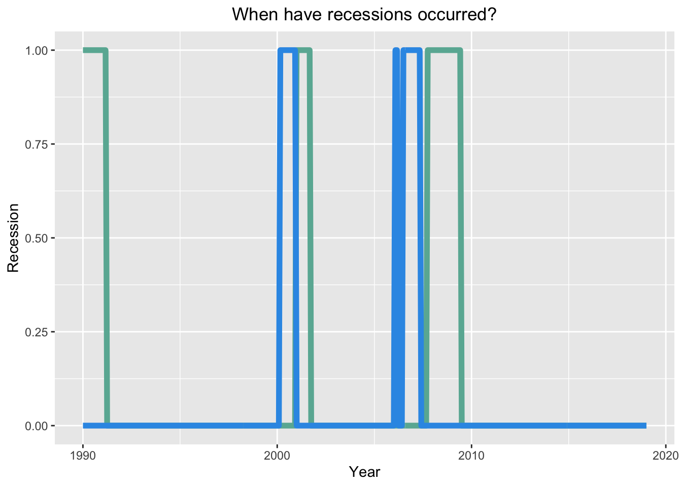
Below is the relationship, between our GDP based recession indicator ‘rec’ and ‘Spread’. To see the relationship we mutated our variable ‘SPREAD’ into a temporary new variable ‘inverted’ (1 if SPREAD<0,0 if SPREAD>0). The green line is ‘rec’ and blue line is ‘inverted’. What we see is that before every recession (green), our ‘inverted’ variable (blue) is present, which indicates that the yield curve is inverted.
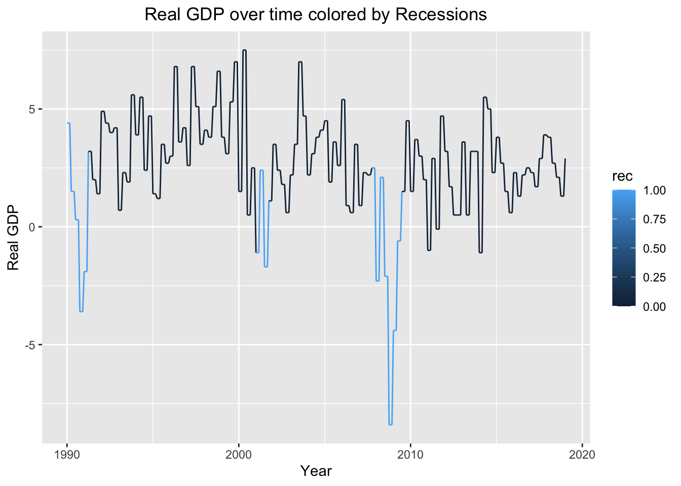
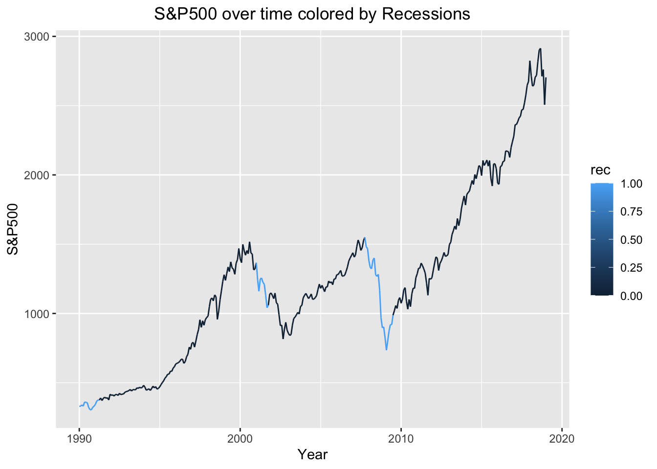
We are also interested in seeing data on real GDP, unemployment rate, and the S&P500 over time, as well as when recessions occurred. For the real GDP plot, whenever a recession occurred and the graph was blue, real GDP dips below 0 and back up. In the S&P500 graph, the graph indicates a recession when the S&P500 declines at a fast rate. However, it is always followed by some kind of rise. This makes sense because a recession is usually followed by economic recovery. When looking at the unemployment graph, a recession is indicated when unemployment increases rapidly. This is not surprising, since during recessions many people lose their jobs and are actively looking for new ones.
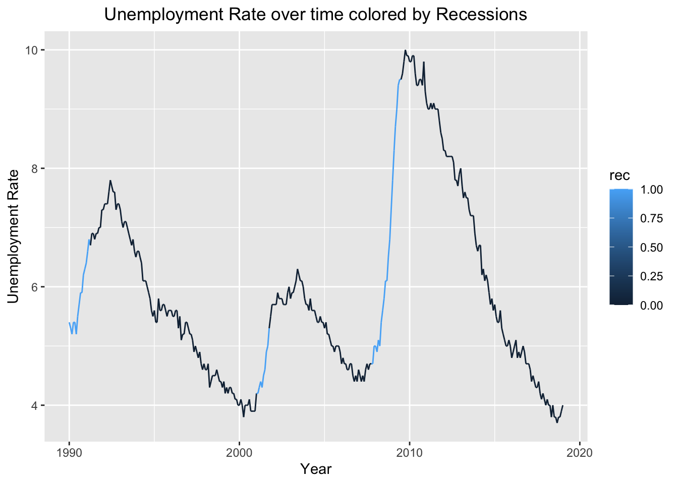
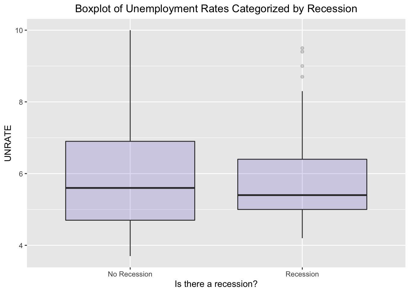
After looking at the time graph of Unemployment rate colored by recession, we also decided to look at a boxplot to compare the mean unemployment rate for when there is a recession and when there isn’t. According to the boxplot, the mean unemployment rate for when there is a recession vs when there isn’t are extremely close, with mean unemployment during a recession being slightly lower. This information is useful for model building.
We performed forward model selection on all of our relevant covariates SPREAD, SP500, GOLD, OIL, CHHUSD, JPYUSD, RGDP, UNRATE, rec, IPI, ‘Copper Price’, ‘Median Income’, BCI, and CCI. The model with the lowest Mallow’s CP is model 7, which is rec~SPREAD+SP500+OIL+JPYUSD+RGDP+IPI+‘Median Income’. Its Mallow’s CP is 58.01230. The variables GOLD, CHHUSD, UNRATE, Copper Price, BCI, and CCI were dropped from the model.
##   (Intercept) SPREAD SP500  GOLD   OIL CHHUSD JPYUSD RGDP UNRATE   IPI
## 1        TRUE  FALSE FALSE FALSE FALSE  FALSE  FALSE TRUE  FALSE FALSE
## 2        TRUE  FALSE FALSE FALSE FALSE  FALSE   TRUE TRUE  FALSE FALSE
## 3        TRUE  FALSE  TRUE FALSE FALSE  FALSE   TRUE TRUE  FALSE FALSE
## 4        TRUE  FALSE  TRUE FALSE  TRUE  FALSE   TRUE TRUE  FALSE FALSE
## 5        TRUE  FALSE  TRUE FALSE  TRUE  FALSE   TRUE TRUE  FALSE FALSE
## 6        TRUE  FALSE  TRUE FALSE  TRUE  FALSE   TRUE TRUE  FALSE  TRUE
## 7        TRUE   TRUE  TRUE FALSE  TRUE  FALSE   TRUE TRUE  FALSE  TRUE
## 8        TRUE   TRUE  TRUE FALSE  TRUE  FALSE   TRUE TRUE   TRUE  TRUE
##   `Copper Price` `Median Income`   BCI   CCI
## 1          FALSE           FALSE FALSE FALSE
## 2          FALSE           FALSE FALSE FALSE
## 3          FALSE           FALSE FALSE FALSE
## 4          FALSE           FALSE FALSE FALSE
## 5          FALSE            TRUE FALSE FALSE
## 6          FALSE            TRUE FALSE FALSE
## 7          FALSE            TRUE FALSE FALSE
## 8          FALSE            TRUE FALSE FALSE
## [1] 252.23525 190.40345 171.92230 131.81356 106.89974 72.15285 58.01230
## [8] 41.15622
We also did an MLR on all of the relevant variables to perform hypothesis testing:
Ho: None of the covariates are significant to the dependent variable
Ha: At least one of the covariates are significant to the dependent variable
With an alpha at 0.01, we see that the variables that aren’t significant are CHHUSD, BCI, and CCI.
##
## Call:
## glm(formula = tempdf2$rec ~ tempdf2$SPREAD + tempdf2$SP500 +
##     tempdf2$GOLD + tempdf2$OIL + tempdf2$CHHUSD + tempdf2$JPYUSD +
##     tempdf2$RGDP + tempdf2$UNRATE + tempdf2$IPI + tempdf2$"Median Income" +
##     tempdf2$"Copper Price" + tempdf2$BCI + tempdf2$CCI, data = tempdf2)
##
## Deviance Residuals:
##      Min        1Q    Median        3Q       Max
## -0.39183  -0.15435  -0.01675   0.10237   0.73833
##
## Coefficients:
##                           Estimate Std. Error t value Pr(>|t|)
## (Intercept)             -5.170e+00  2.538e+00  -2.037 0.042460 *
## tempdf2$SPREAD          -2.233e-01  5.776e-02  -3.866 0.000133 ***
## tempdf2$SP500           -5.664e-04  8.378e-05  -6.761 6.10e-11 ***
## tempdf2$GOLD             4.544e-04  1.103e-04   4.119 4.80e-05 ***
## tempdf2$OIL              1.231e-02  1.391e-03   8.849  < 2e-16 ***
## tempdf2$CHHUSD           1.516e-01  1.269e-01   1.195 0.232875
## tempdf2$JPYUSD           4.893e-03  1.122e-03   4.363 1.71e-05 ***
## tempdf2$RGDP            -6.435e-02  5.313e-03 -12.111  < 2e-16 ***
## tempdf2$UNRATE          -9.616e-02  1.708e-02  -5.630 3.81e-08 ***
## tempdf2$IPI             -1.140e-02  3.666e-03  -3.109 0.002036 **
## tempdf2$"Median Income"  8.121e-05  1.215e-05   6.685 9.67e-11 ***
## tempdf2$"Copper Price"  -6.141e-05  2.036e-05  -3.017 0.002751 **
## tempdf2$BCI             -2.334e-02  1.234e-02  -1.891 0.059439 .
## tempdf2$CCI              3.880e-02  1.865e-02   2.081 0.038199 *
## ---
## Signif. codes:  0 '***' 0.001 '**' 0.01 '*' 0.05 '.' 0.1 ' ' 1
##
## (Dispersion parameter for gaussian family taken to be 0.04611698)
##
##     Null deviance: 39.198  on 348  degrees of freedom
## Residual deviance: 15.449  on 335  degrees of freedom
## AIC: -67.594
##
## Number of Fisher Scoring iterations: 2
By analyzing the variable selection output and MLR output, we decided to fit our final model through the Mallow’s CP method because it dropped the same insignificant variables as the MLR method but also dropped more. This will make our model more accurate.
Our final model is rec~SPREAD+SP500+OIL+JPYUSD+RGDP+IPI+‘Median Income’.
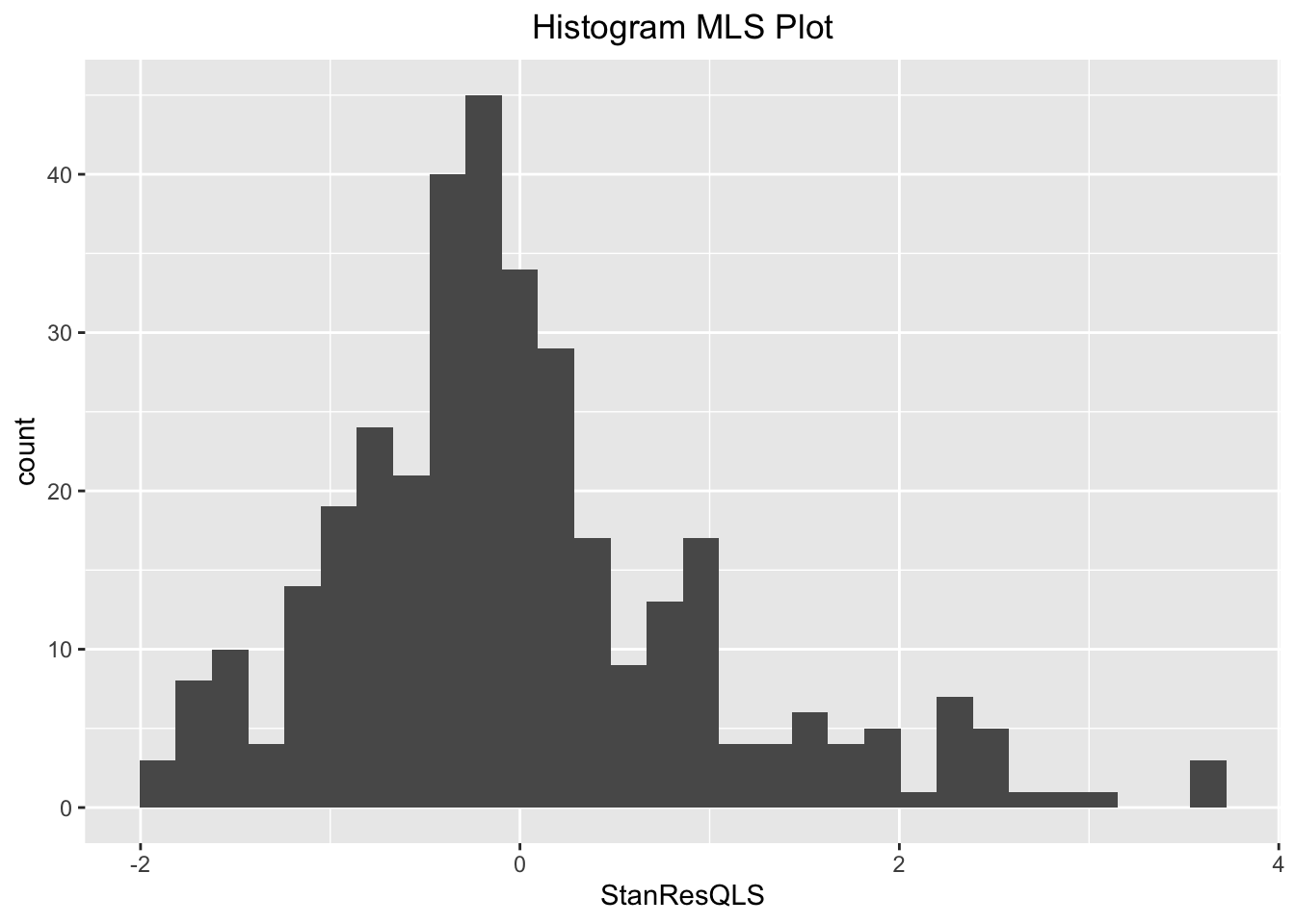
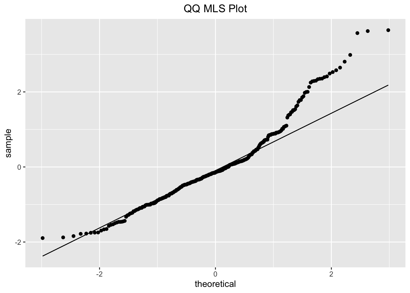
We also decided to test for normality of this new model. From both the histogram and QQ plot, we see that the data is skewed right. However, the histogram is unimodal and the QQ plot is roughly straight, we decided to assume that the model is approximately normal and proceed with linear testing.
After fitting a linear model, we can reject a null hypothesis that there is no relationship between the dependent variable rec and our covariates becuase the model p-value is close to 0. In this summary table, it is shown that every variable is significant with a p-value<0.01.
##
## Call:
## lm(formula = tempdf2$rec ~ tempdf2$SPREAD + tempdf2$SP500 + tempdf2$OIL +
##     tempdf2$JPYUSD + tempdf2$RGDP + tempdf2$IPI + tempdf2$"Median Income")
##
## Residuals:
##      Min       1Q   Median       3Q      Max
## -0.43236 -0.13932 -0.03203  0.09581  0.83440
##
## Coefficients:
##                           Estimate Std. Error t value Pr(>|t|)
## (Intercept)             -4.433e+00  5.130e-01  -8.641  < 2e-16 ***
## tempdf2$SPREAD          -1.971e-01  5.253e-02  -3.752 0.000206 ***
## tempdf2$SP500           -2.657e-04  4.378e-05  -6.069 3.42e-09 ***
## tempdf2$OIL              8.156e-03  8.694e-04   9.381  < 2e-16 ***
## tempdf2$JPYUSD           5.971e-03  1.038e-03   5.751 1.97e-08 ***
## tempdf2$RGDP            -6.506e-02  5.464e-03 -11.906  < 2e-16 ***
## tempdf2$IPI             -1.623e-02  3.003e-03  -5.405 1.22e-07 ***
## tempdf2$"Median Income"  9.228e-05  1.157e-05   7.978 2.29e-14 ***
## ---
## Signif. codes:  0 '***' 0.001 '**' 0.01 '*' 0.05 '.' 0.1 ' ' 1
##
## Residual standard error: 0.23 on 341 degrees of freedom
## Multiple R-squared:   0.54,  Adjusted R-squared:  0.5305
## F-statistic: 57.18 on 7 and 341 DF,  p-value: < 2.2e-16
The original thesis of this project was how we can predict a recession. However, we acknowledged that it is not entirely possible. So much randomness and external factors occur that aren’t always easy to measure mathematically. We also acknowledge that it isn’t totally necessary to fit a linear model that can predict recessions, and that the model isn’t totally accurate. However, it helped show us the relationship between different economic indicators and the occurrence of a recession, which ultimately helped us answer our thesis.